Google Summer of Code 2013

Google Summer of Code (GSoC) 2013 was an absolute blast! The majority of my heavy coding is over so I wanted to post a bit about the experience. It has been fantastic I’ve learned so much and done so many different and unexpected things. And before I go any further I want to give a big thanks to all the Shogun devs who helped me out and made this program so great and also thanks to Google for running such a kick ass program.

My project was to code several Independent Component Analysis (ICA) algorithms specifically those based on Approximate Joint Diagonalization (ADJ) of matrices. The application is for Blind Source Separation (BSS) - think the cocktail party problem. It was pretty cool and similar enough to my thesis work that I was able to jump right in fairly quickly. It was an interesting change of pace for me, as I like to put it: it’s called Google Summer of Code not Google Summer of Research and having the code be the number one priority was a welcome change of pace for me. As the focus was code I spent a lot of time translating research papers and author’s source code into production code. I like to think I am quite the wizz with porting between numerical libraries now (matlab -> python,  python -> c etc.) Also I’m now so familiar with NumPy, Octave and Eigen3 (and almost R) that I can pretty much work fluently in each and change between them quickly almost without noticing. Have a look at my recent post One Example Three Languages!

One of the other things I got into this summer was playing with the Shogun Modular interfaces which are created using SWIG. I once tried to play with SWIG for one of my own projects but unfortunately never got far. This summer though I updated a few of the typemaps to add support for NDArray which some of my classes needed. I also playing with updating the ruby modular interface to use the newer and more active NMatrix numerical library (not included in Shogun as of yet though). Anyways playing with typemaps was an interesting experience and I definitely learned more than a few things.

One of the other things I learned was the softer side of class and framework design. I realized that even though I’ve been doing OOP for years one thing I still need more experience with is laying out a new class from scratch. The first time I had to do this I actually had to stop for a second and think, I actually wrote a basic foo bar style class example to double check that what I wanted to do would work. In the end I am quite happy with the class structure I came up with and I look forward to being involved in this type of design more often in the future.

Thats all I can think of now! If you’re a student I highly recommend doing GSoC!

Also here is a link to my final project:

http://nbviewer.ipython.org/urls/raw.github.com/pickle27/bss_jade/master/bss_jade.ipynb
One Example Three Languages

I wanted to post this example of my Google Summer of Code work because I think it’s neat. One of the cool things about Shogun is our great SWIG wrapper and our static interface which lets us use Shogun natively in a bunch of different languages. So here is an example program of doing Blind Source Separation using the Jade algorithm from Python, Octave and R:

"""
Blind Source Separation using the Jade Algorithm with Shogun
Based on the example from scikit-learn
http://scikit-learn.org/

Kevin Hughes 2013
"""

import numpy as np
import pylab as pl

from shogun.Features  import RealFeatures
from shogun.Converter import Jade

# Generate sample data
np.random.seed(0)
n_samples = 2000
time = np.linspace(0, 10, n_samples)

# Source Signals
s1 = np.sin(2 * time)  # sin wave
s2 = np.sign(np.sin(3 * time))  # square wave
S = np.c_[s1, s2]
S += 0.2 * np.random.normal(size=S.shape)  # add noise

# Standardize data
S /= S.std(axis=0)  
S = S.T

# Mixing Matrix
A = np.array([[1, 0.5], [0.5, 1]])

# Mix Signals
X = np.dot(A,S)
mixed_signals = RealFeatures(X)

# Separating
jade = Jade()
signals = jade.apply(mixed_signals)
S_ = signals.get_feature_matrix()
A_ = jade.get_mixing_matrix();

# Plot results
pl.figure()
pl.subplot(3, 1, 1)
pl.plot(S.T)
pl.title('True Sources')
pl.subplot(3, 1, 2)
pl.plot(X.T)
pl.title('Mixed Sources')
pl.subplot(3, 1, 3)
pl.plot(S_.T)
pl.title('Estimated Sources')
pl.subplots_adjust(0.09, 0.04, 0.94, 0.94, 0.26, 0.36)
pl.show()
% Blind Source Separation using the Jade Algorithm with Shogun
%
% Based on the example from scikit-learn
% http://scikit-learn.org/
%
% Kevin Hughes 2013

% Generate sample data
n_samples = 2000;
time = linspace(0,10,n_samples);

% Source Signals
S = zeros(2, length(time));
S(1,:) = sin(2*time);
S(2,:) = sign(sin(3*time));
S += 0.2*rand(size(S));

% Standardize data
S = S ./ std(S,0,2);

% Mixing Matrix
A = [1 0.5; 0.5 1]

% Mix Signals
X = A*S;
mixed_signals = X;

% Separating
sg('set_converter', 'jade');
sg('set_features', 'TRAIN', mixed_signals);
S_ = sg('apply_converter');

% Plot
figure();
subplot(311);
plot(time, S(1,:), 'b');
hold on;
plot(time, S(2,:), 'g');
set(gca, 'xtick', [])
title("True Sources");

subplot(312);
plot(time, X(1,:), 'b');
hold on;
plot(time, X(2,:), 'g');
set(gca, 'xtick', [])
title("Mixed Sources");

subplot(313);
plot(time, S_(1,:), 'b');
hold on;
plot(time, S_(2,:), 'g');
title("Estimated Sources");
# Blind Source Separation using the Jade Algorithm with Shogun
#
# Based on the example from scikit-learn
# http://scikit-learn.org/
#
# Kevin Hughes 2013

library('sg')

# Generate sample data
n_samples <- 2000
time <- seq(0,10,length=n_samples)

# Source Signals
S <- matrix(0,2,n_samples)
S[1,] <- sin(2*time)
S[2,] <- sign(sin(3*time))
S <- S + 0.2*matrix(runif(2*n_samples),2,n_samples)

# Standardize data
S <- S * (1/apply(S,1,sd))

# Mixing Matrix
A <- rbind(c(1,0.5),c(0.5,1))

# Mix Signals
X <- A %*% S
mixed_signals <- matrix(X,2,n_samples)

# Separating
sg('set_converter', 'jade')
sg('set_features', 'TRAIN', mixed_signals)
S_ <- sg('apply_converter')

# Plot
par(mfcol=c(3,1));

plot(time, S[1,], type="l", col='blue', main="True Sources", ylab="", xlab="")
lines(time, S[2,], type="l", col='green')

plot(time, X[1,], type="l", col='blue', main="Mixed Sources", ylab="", xlab="")
lines(time, X[2,], type="l", col='green')

plot(time, S_[1,], type="l", col='blue', main="Estimated Sources", ylab="", xlab="")
lines(time, S_[2,], type="l", col='green')

Successfully Defended my Thesis!

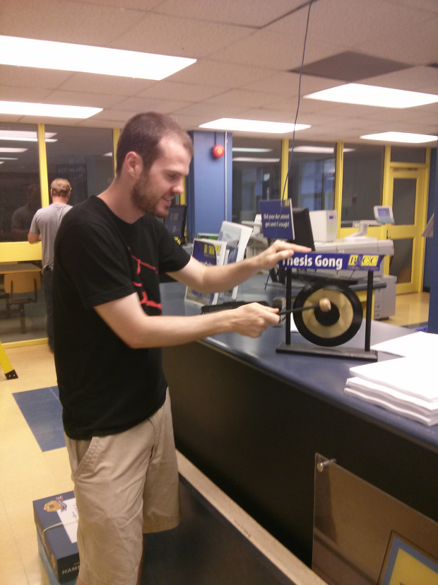
Hitting the thesis gong in the Queen's Print center when I submitted last month

After 2 long and intense years of work yesterday I defended my thesis titled Subspace Bootstrapping and Learning for Background Subtraction. Grad School has been a blast but I’m definitely looking forward to employed life!

I’ll post a link to my thesis under publications as soon as Queen’s uploads it to their system.

*edit* the link to my thesis is on my publications page